Manual structural analysis of a continuous beam using the method of singularity functions (Macaulay’s method)

Singularity functions are a mathematical tool used to describe systems where discontinuity occurs. These functions are written using a special notation using singularity brackets: $\langle \rangle$ . The general functions is written as $\langle x-a \rangle^n$ where $a$ is the point of discontinuity and $n$ is the function degree. A detailed explanation of the properties of these functions can be found on Wikipedia.
The singularity functions method is sometimes refereed to as “Macaulay’s method” and the brackets as “Macaulay brackets”.

The main advantage of using singularity functions for solving the continuous beam problem is the ability to describe and solve the system analytically with any kind of load. This can be done for complex loading systems such as having the load described as a high order function. The symbolic solution can be reached without any approximation which gives us a pure analytical solution to any continuous beam.

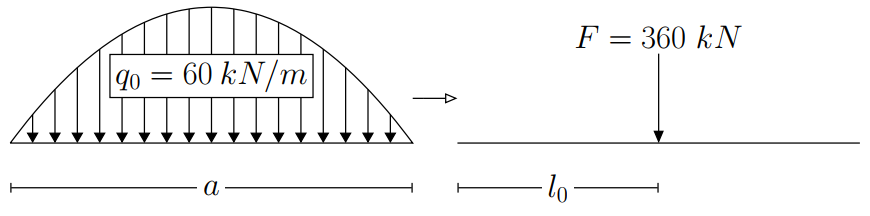
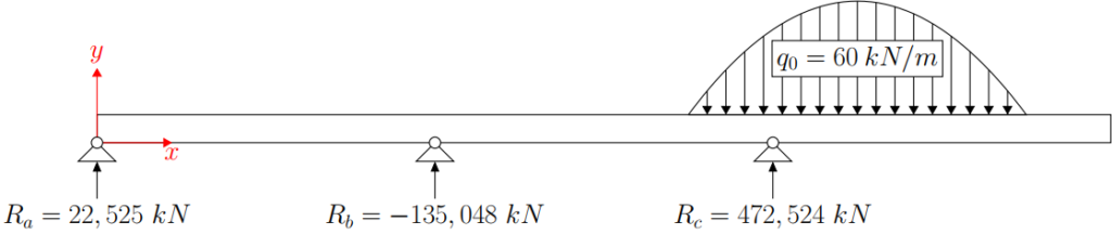
To demonstrate this, the following continuous beam is used as an example:

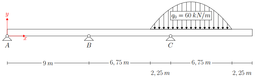
Continuous beam problem (lengths in meter)

The load is described as a function of the length $x$ starting at $x=15.75$ to $x= 24.75$ from left to right. Equation (1) describes the load function; where: $q_0 = 60 kN$ and $a = 9 m$ .

(1) $\begin{equation*} q(x)=-\frac{4q_0}{a^2} x^2 + \frac{4q_0}{a} x \end{equation*}$

First we should determine the reaction forces Ra, Rb and Rc.

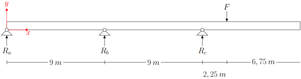
This is done by simplifying the load as follows:

(2) $\begin{equation*} \begin{array}{l} q(x)=-\frac{4 q_{0}}{a^{2}} x_{0}^{2}+\frac{4 q_{0}}{a} x_{0} \\ F=\int_{0}^{9} q(x) d x=6 q_{0}=360 k N \\ l_{0}=\frac{\int_{0}^{9} q(x) x d x}{F}=4,5 m \end{array} \end{equation*}$

Using simple static we can determine the system equations 3 and 4 .

(3) $\begin{equation*} \sum F_y=0 \rightarrow Ra+Rb+Rc=6 q_{0} \end{equation*}$

(4) $\begin{equation*} \sum Mc=0 \rightarrow Rb+2Rc=13.5 q_{0} \end{equation*}$

We start the solution by writing the equation of normal forces as shown in 5. To get the equation, a couple of rules should be known: for single loads we use a singularity function with a degree of $n=-1$ , constant line loads get a degree of $n=0$ and so on. Rules in applying singularity functions can be seen in this link.
The challenge occurs when having loads with higher order $n>=2$ (such as the one in our example). In this case the load should be described as a Taylor expansion. The reason for this is explained in this discussion.

(5) $\begin{align*} \begin{split} q(x)&=Ra<x-0>^{-1}+Rb<x-9>^{-1}+Rc<x-18>^{-1}\\ &+\frac{4q_{0}}{9}<x-15.75>^{1}-\frac{4 q_{0}}{81}<x-15.75>^{2} \end{split} \end{align*}$

Now we actually finished the most important part on the solution and the rest is simple mathematics!
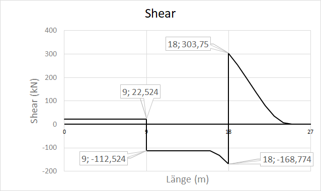
To get the shear force equation, we integrate the force equation 5 as seen in equation 6

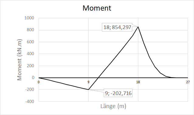
(6) $\begin{align*} \begin{split} V(x)&=\int q(x)dx\\ V(x)&=Ra<x-0>^{0}+Rb<x-9>^{0}+Rc<x-18>^{0}\\ &+\frac{4q_{0}}{18}<x-15.75>^{2}-\frac{4 q_{0}}{243}<x-15.75>^{3} \end{split} \end{align*}$

Similarly we get the bending moment equation 7.

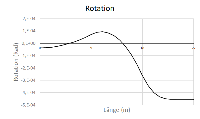
(7) $\begin{align*} \begin{split} M(x)&=\int V(x)dx\\ M(x)&=Ra<x-0>^{1}+Rb<x-9>^{1}+Rc<x-18>^{1}\\ &+\frac{4q_{0}}{54}<x-15.75>^{3}-\frac{4 q_{0}}{972}<x-15.75>^{4} \end{split} \end{align*}$

Rotation is calculated in 8. Here we should take an integration constant $C_1$ into account. This is due to the fact, that the rotation at the $x=0$ doesn’t equal 0.

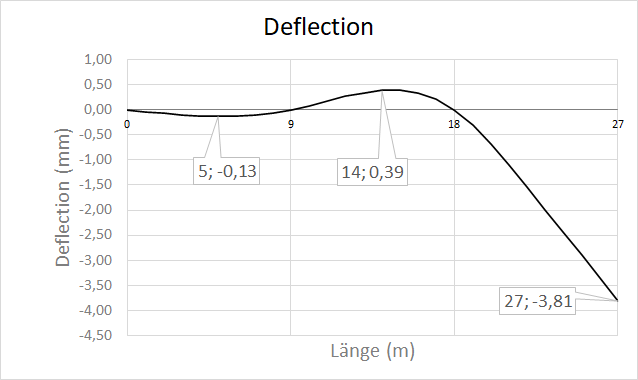
(8) $\begin{align*} \begin{split} EI\theta(x)&=\int M(x)dx\\ EI\theta(x)&=\frac{Ra}{2}<x-0>^{2}+\frac{Rb}{2}<x-9>^{2}+\frac{Rc}{2}<x-18>^{2}\\ &+\frac{4q_{0}}{216}<x-15.75>^{4}-\frac{4 q_{0}}{4860}<x-15.75>^{5}+C_1 \end{split} \end{align*}$

Finally we can derive the deflection equation as in 9.

(9) $\begin{align*} \begin{split} EIy(x)&=\int EI\theta(x)dx\\ EIy(x)&=\frac{Ra}{6}<x-0>^{3}+\frac{Rb}{6}<x-9>^{3}+\frac{Rc}{6}<x-18>^{3}\\ &+\frac{4q_{0}}{1080}<x-15.75>^{5}-\frac{4 q_{0}}{4860}<x-15.75>^{6}+C_1*x \end{split} \end{align*}$

Determining $C_1$ : when $x=9$ then $EIy(9) = 0$ therefore by substituting in the deflection equation we determine the following:

$0=\frac{R a}{6}<9-0>^{3}+9C_{1} \rightarrow C_{1}=-13.5 Ra$

When $x=18$ then $EIy(18) = 0$ therefore by substituting in the deflection equation we determine 10.

(10) $\begin{equation*} 729 Ra+121.5 Rb=\left(\frac{8019}{40960}\right) q_{0} \end{equation*}$

Now by solving equations 3,4 and 10 we can determine the reaction forces:

(11) $\begin{align*} Ra&=\left(\frac{30753}{81920}\right) q_{0} \\ Rb&=-\left(\frac{92193}{40960}\right) q_{0} \\ Rc&=\left(\frac{645153}{40960}\right) q_{0} \\ q_{0}&=60\ kN/m \rightarrow \\ Ra&=22.524\ kN \\ Rb&=-135.048\ kN \\ Rc&=472.524\ kN \end{align*}$

Since we already determined the equations of the internal forces and calculated the reactions, we can simply plot the equations by varying the value of $x$ .

The following is the VBA code used to plot the solution. It can be used as a reference on the proper way to implement singularity functions in VBA/Excel.

Public Const Ra = 22.524
Public Const Rb = -135.048
Public Const Rc = 472.524
Public Const q0 = 60
Public Const E = 2.1 * 10 ^ 8
Public Const I = 3945001.5 * 10 ^ -8
Public Const EI = E * I

Function Shear(x)
    y1 = Abs(x >= 0) * Ra * (x - 0) ^ 0
    y2 = Abs(x >= 9) * Rb * (x - 9) ^ 0
    y3 = Abs(x >= 18) * Rc * (x - 18) ^ 0
    y4 = Abs(x >= 15.75) * (-4 * q0 / 18) * (x - 15.75) ^ 2
    y5 = Abs(x >= 15.75) * (4 * q0 / 243) * (x - 15.75) ^ 3
    
    Shear = Abs(x <= 24.75) * (y1 + y2 + y3 + y4 + y5)
End Function

Function Moment(x)
    y1 = Abs(x >= 0) * Ra * (x - 0) ^ 1
    y2 = Abs(x >= 9) * Rb * (x - 9) ^ 1
    y3 = Abs(x >= 18) * Rc * (x - 18) ^ 1
    y4 = Abs(x >= 15.75) * (-4 * q0 / 54) * (x - 15.75) ^ 3
    y5 = Abs(x >= 15.75) * (4 * q0 / 972) * (x - 15.75) ^ 4
    
    Moment = -Abs(x <= 24.75) * (y1 + y2 + y3 + y4 + y5)
End Function

Function Rotation(x)
    If x > 24.75 Then
        Rotation = Rotation(24.75)
        Exit Function
    End If
    
    y1 = Abs(x >= 0) * (1 / 2) * Ra * (x - 0) ^ 2
    y2 = Abs(x >= 9) * (1 / 2) * Rb * (x - 9) ^ 2
    y3 = Abs(x >= 18) * (1 / 2) * Rc * (x - 18) ^ 2
    y4 = Abs(x >= 15.75) * (-4 * q0 / 216) * (x - 15.75) ^ 4
    y5 = Abs(x >= 15.75) * (4 * q0 / 4860) * (x - 15.75) ^ 5
    y6 = -13.5 * Ra
    
    EItheta = Abs(x <= 24.75) * (y1 + y2 + y3 + y4 + y5 + y6)
    Rotation = EItheta / EI
End Function

Function Deflection(x)
    
    If x > 24.75 Then
        Deflection = Deflection(24.75) + Rotation(24.75) * (x - 24.75)
        Exit Function
    End If
    
    y1 = Abs(x >= 0) * (1 / 6) * Ra * (x - 0) ^ 3
    y2 = Abs(x >= 9) * (1 / 6) * Rb * (x - 9) ^ 3
    y3 = Abs(x >= 18) * (1 / 6) * Rc * (x - 18) ^ 3
    y4 = Abs(x >= 15.75) * (-4 * q0 / 1080) * (x - 15.75) ^ 5
    y5 = Abs(x >= 15.75) * (4 * q0 / 29160) * (x - 15.75) ^ 6
    y6 = -13.5 * Ra * x
    
    EIy = Abs(x <= 24.75) * (y1 + y2 + y3 + y4 + y5 + y6)
    Deflection = EIy / EI
    
End Function

Related Posts

Leave a Comment Cancel Reply