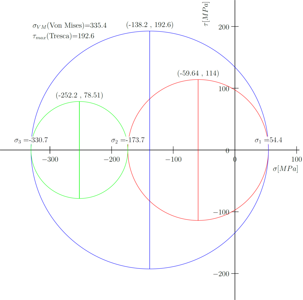
This is a simple script in Asymptote to plot Mohr’s Circle for 3D stress analysis
(Also available on GitHub)
import graph;
import settings;
settings.outformat = "pdf";

//Inputs start

//defaultpen(fontsize(5pt));
string m_unit = "MPa";
real unit_step = 100;

real s_x = -100;
real s_y = -200;
real s_z = -150;
real t_xy = 50;
real t_xz = 100;
real t_yz = 150;


// real s_x = 120;
// real s_y = -85;
// real s_z = 0.0001;
// real t_xy = -80;
// real t_xz = 1;
// real t_yz = 1;


//Inputs end

// Stress Invariants
//https://en.wikiversity.org/wiki/Introduction_to_Elasticity/Principal_stresses

real I_1 = s_x+s_y+s_z;
real I_2 = s_x*s_y+s_y*s_z+s_z*s_x-t_xy**2-t_xz**2-t_yz**2;
real I_3=(s_x*s_y*s_z)-s_x*t_yz**2-s_y*t_xz**2-s_z*t_xy**2+(2*t_xy*t_xz*t_yz);

real phi = (1/3)*acos((2*I_1**3-9*I_1*I_2+27*I_3)/(2*(I_1**2-3*I_2)**(3/2)));


// Principal Stresses

real s_1=(I_1/3)+(2/3)*sqrt(I_1**2-3*I_2)*cos(phi);

real s_2=(I_1/3)+(2/3)*sqrt(I_1**2-3*I_2)*cos(phi-2*pi/3);

real s_3=(I_1/3)+(2/3)*sqrt(I_1**2-3*I_2)*cos(phi-4*pi/3);


// Circles

real C_1= 0.5*(s_1+s_2);
real C_2= 0.5*(s_1+s_3);
real C_3= 0.5*(s_2+s_3);

real R_1= 0.5*(s_1-s_2);
real R_2= 0.5*(s_1-s_3);
real R_3= 0.5*(s_2-s_3);

//size(6cm);

path c1= circle((C_1,0),R_1);
path c2= circle((C_2,0),R_2);
path c3= circle((C_3,0),R_3);

draw(c1,red);
draw(c2,blue);
draw(c3,green);


// fill(circle((C_1,R_1),2pt),red);
// fill(circle((C_2,R_2),2pt),blue);
// fill(circle((C_3,R_3),2pt),green);

draw((C_1,R_1)--(C_1,-R_1),red);
draw((C_2,R_2)--(C_2,-R_2),blue);
draw((C_3,R_3)--(C_3,-R_3),green);
// real[] tabT={C_1,C_2,C_3,s_1,s_2,s_3};
real[] tabT={0};

xaxis(L="$\sigma ["+m_unit+"]$", axis=YZero,xmin=s_3-50, xmax=s_1+50, ticks=Ticks(Step=unit_step));
yaxis(L="$\tau ["+m_unit+"]$", axis=XZero,ymin=-R_2-50, ymax=R_2+50 , ticks=Ticks(Step=unit_step));

label(L="$\sigma_1="+format(s_1)+"$",position=(s_1,0),N*3,filltype=Fill(white+opacity(0.9)));
label(L="$\sigma_2="+format(s_2)+"$",position=(s_2,0),N*3,filltype=Fill(white+opacity(0.9)));
label(L="$\sigma_3="+format(s_3)+"$",position=(s_3,0),N*3,filltype=Fill(white+opacity(0.9)));


label(L="$("+format(C_1)+"\ ,\ "+format(R_1)+")$",position=(C_1,R_1),N);
label(L="$("+format(C_2)+"\ ,\ "+format(R_2)+")$",position=(C_2,R_2),N);
label(L="$("+format(C_3)+"\ ,\ "+format(R_3)+")$",position=(C_3,R_3),N);

real s_vm=sqrt(0.5*((s_1-s_3)**2+(s_2-s_3)**2+(s_1-s_2)**2));

label(L="$\sigma_{VM}$(Von Mises)="+format(s_vm),position=(s_3,R_2),NE);
label(L="$\tau_{max}$(Tresca)="+format(R_2),position=(s_3,R_2),SE);
The following picture shows the results of executing this script.